In this post, I will analyse the #Tidytuesday Dataset about a video game from the Steam store.

Load the packages
library(tidyverse)
library(lubridate)
library(magrittr)
library(ggthemr)
library(RColorBrewer)
library(gganimate)
Load the data
video_game <-
  read_csv("https://raw.githubusercontent.com/rfordatascience/tidytuesday/master/data/2019/2019-07-30/video_games.csv")
Data Transformation
Lets take a look at our dataframe.
# A tibble: 6 x 10
  number game  release_date price owners developer publisher
   <dbl> <chr> <chr>        <dbl> <chr>  <chr>     <chr>
1      1 Half~ Nov 16, 2004  9.99 10,00~ Valve     Valve
2      3 Coun~ Nov 1, 2004   9.99 10,00~ Valve     Valve
3     21 Coun~ Mar 1, 2004   9.99 10,00~ Valve     Valve
4     47 Half~ Nov 1, 2004   4.99 5,000~ Valve     Valve
5     36 Half~ Jun 1, 2004   9.99 2,000~ Valve     Valve
6     52 CS2D  Dec 24, 2004 NA    1,000~ Unreal S~ Unreal S~
# ... with 3 more variables: average_playtime <dbl>,
# median_playtime <dbl>, metascore <dbl> number game release_date
Min. : 1 Length:26688 Length:26688
1st Qu.: 821 Class :character Class :character
Median :2356 Mode :character Mode :character
Mean :2904
3rd Qu.:4523
Max. :8846
price owners developer
Min. : 0.490 Length:26688 Length:26688
1st Qu.: 2.990 Class :character Class :character
Median : 5.990 Mode :character Mode :character
Mean : 8.947
3rd Qu.: 9.990
Max. :595.990
NA's :3095
publisher average_playtime median_playtime
Length:26688 Min. : 0.000 Min. : 0.00
Class :character 1st Qu.: 0.000 1st Qu.: 0.00
Mode :character Median : 0.000 Median : 0.00
Mean : 9.057 Mean : 5.16
3rd Qu.: 0.000 3rd Qu.: 0.00
Max. :5670.000 Max. :3293.00
NA's :9 NA's :12
metascore
Min. :20.00
1st Qu.:66.00
Median :73.00
Mean :71.89
3rd Qu.:80.00
Max. :98.00
NA's :23838 video_game dataframe has 26688 rows and 10 columns.
Missing value
Lets check for the missing value in the dataframe.
          number             game     release_date            price
               0                3                0             3095
          owners        developer        publisher average_playtime
               0              151               95                9
 median_playtime        metascore
              12            23838
Above output shows that We have missing value in this data frame. We will use the median value to replace the missing value of numerical columns.
video_game <- video_game %>% mutate(metascore = replace(
  metascore,
  is.na(metascore),
  median(metascore, na.rm = TRUE)
))

video_game <- video_game %>% mutate(price = replace(
  price,
  is.na(price),
  median(price, na.rm = TRUE)
))

video_game <- video_game %>% mutate(average_playtime = replace(
  average_playtime,
  is.na(average_playtime),
  median(average_playtime, na.rm = TRUE)
))

video_game <- video_game %>% mutate(median_playtime = replace(
  median_playtime,
  is.na(median_playtime),
  median(median_playtime, na.rm = TRUE)
))
video_game <- video_game %>% mutate(
year = year(mdy(release_date)),
month = month(mdy(release_date), label = TRUE),
weekday = wday(mdy(release_date), label = TRUE)
) number game release_date price
0 0 0 0
owners developer publisher average_playtime
0 0 0 0
median_playtime metascore year month
0 0 0 0
weekday
0 We replaced the numerical values with the median of the respective values and dropped the missing rows in publisher and developer column.
video_game %<>%
  mutate(
    max_owners = str_trim(word(owners, 2, sep = "\\..")),
    max_owners = as.numeric(str_replace_all(max_owners, ",", "")),
    min_owners = str_trim(word(owners, 1, sep = "\\..")),
    min_owners = as.numeric(str_replace_all(min_owners, ",", ""))
  )
The owner column has the range of owner of a game and the code create max and min owner of the game.
Let’s see the final data frame:
# A tibble: 6 x 15
  number game  release_date price owners developer publisher
   <dbl> <chr> <chr>        <dbl> <chr>  <chr>     <chr>
1      1 Half~ Nov 16, 2004  9.99 10,00~ Valve     Valve
2      3 Coun~ Nov 1, 2004   9.99 10,00~ Valve     Valve
3     21 Coun~ Mar 1, 2004   9.99 10,00~ Valve     Valve
4      2 Unre~ Mar 16, 2004 15.0  500,0~ Epic Gam~ Epic Gam~
5      4 DOOM~ Aug 3, 2004   4.99 500,0~ id Softw~ id Softw~
6     14 Beyo~ Apr 27, 2004  5.99 500,0~ Larian S~ Larian S~
# ... with 8 more variables: average_playtime <dbl>,
#   median_playtime <dbl>, metascore <dbl>, year <dbl>, month <ord>,
#   weekday <ord>, max_owners <dbl>, min_owners <dbl>
Visualization of Data
discrete_pal <- c(
  "#fa4234", "#f5b951", "#e8f538", "#52b0f7",
  "#b84ef5", "#4ed1f5", "#45b58e", "#1a1612",
  "#474ccc", "#47cc92", "#a0cc47", "#c96f32"
)ggthemr("flat")
ggplot(data = video_game %>% group_by(developer) %>%
tally(sort = TRUE) %>% head(10)) +
geom_col(aes(x = reorder(developer, n), y = n, fill = n)) +
labs(
title = "Developer with most Games", x = NULL, y = "Game Count",
fill = "Game Count", caption = "by: @diwastha"
) +
theme_minimal() +
theme(axis.text.x = element_text(angle = 40, hjust = 1))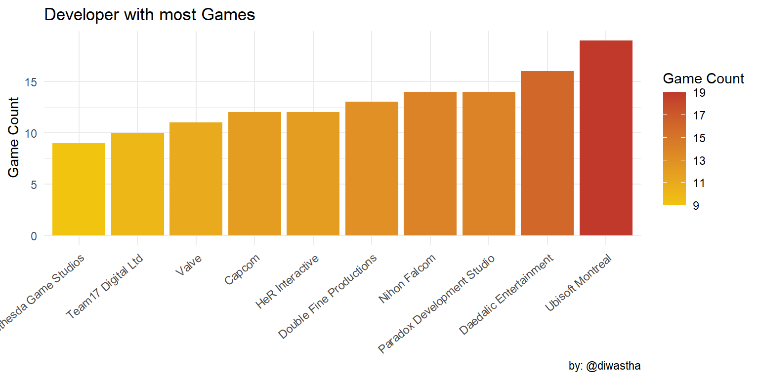
ggplot(data = video_game %>% group_by(publisher) %>%
  tally(sort = TRUE) %>% head(10)) +
  geom_col(aes(x = reorder(publisher, n), y = n, fill = n)) +
  labs(
    title = "Publisher with most Games", y = "Game Count", x = NULL,
    fill = "Game Count", caption = "by: @diwastha"
  ) +
  theme_minimal() +
  theme(axis.text.x = element_text(angle = 40, hjust = 1))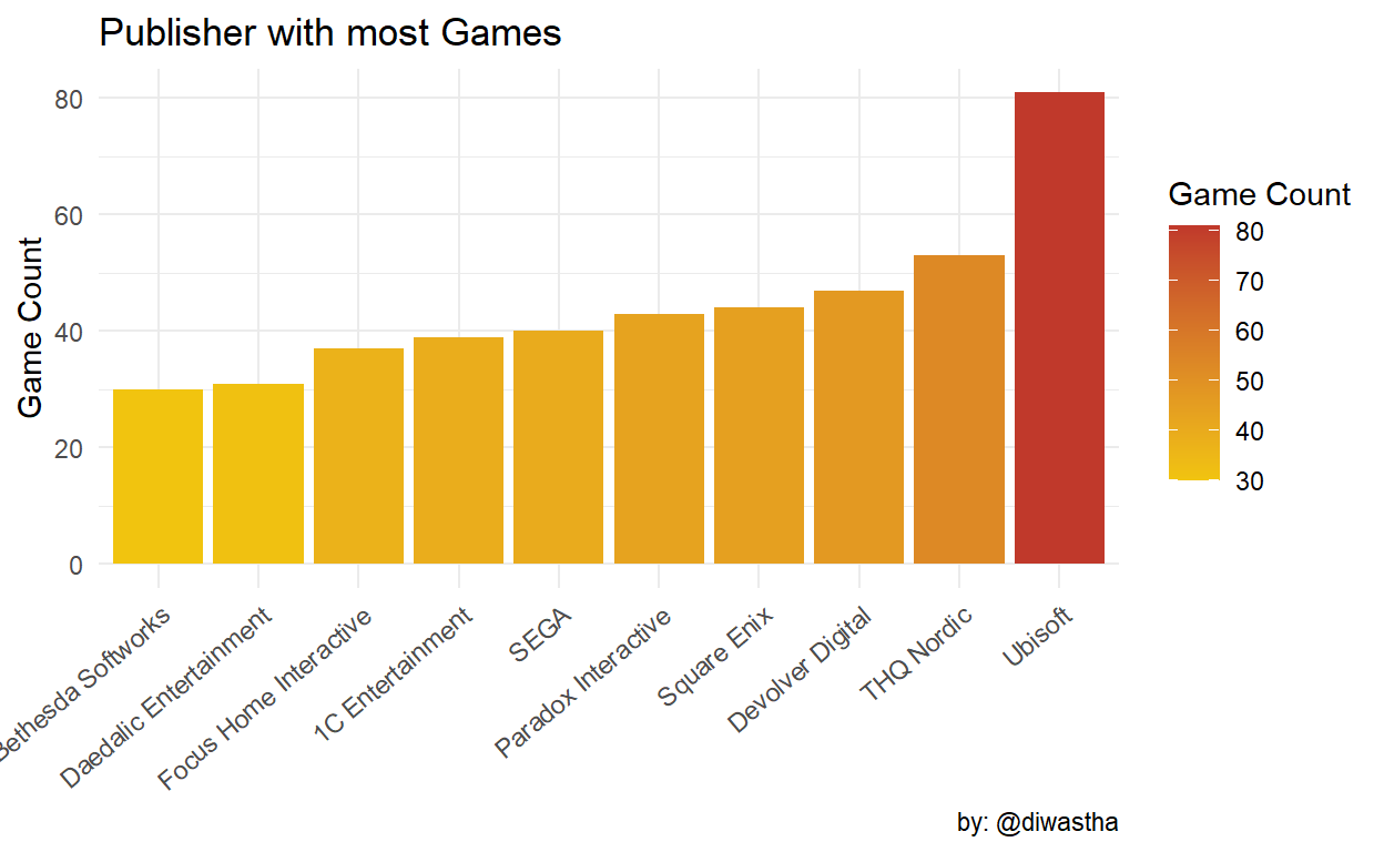
Big Fish Games is the biggest publisher by the game count as it publishes lots of free to play and casual games. Sega which is the second-largest publisher has less than half of the game published by the Big Fish Games.
video_game %>%
  select(-number) %>%
  mutate(max_owners = as.factor(max_owners / 1000000)) %>%
  group_by(publisher) %>%
  mutate(n = n()) %>%
  ungroup() %>%
  filter(n >= 80) %>%
  ggplot(aes(publisher, max_owners, color = publisher)) +
  geom_jitter(show.legend = FALSE, size = 2, alpha = 0.5) +
  labs(
    title = "Distribution of ownership of top publishers",
    y = "Estimated Game Ownership per Million", x = NULL
  ) +
  theme_minimal() + scale_color_manual(values = discrete_pal) +
  theme(axis.text.x = element_text(angle = 45, hjust = 1)) +
  stat_summary(
    fun.y = mean, geom = "line", shape = 20,
    size = 5, color = "#555555"
  )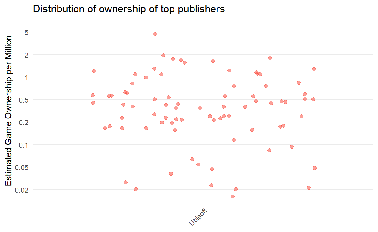
The Big Fish Games has released 265 games but the player base of their games is very small. Other publishers in this group have a much larger player base like Ubisoft, Square Enix, SEGA has much larger player base for their games.
ggplot(data = video_game %>% arrange(desc(average_playtime)) %>% head(20)) +
  geom_col(aes(x = reorder(game, average_playtime), y = average_playtime, fill = metascore)) +
  labs(
    title = "Games with most metascore", x = NULL, y = "Average Playtime",
    caption = "by: @diwastha"
  ) +
  theme_minimal() +
  theme(axis.text.x = element_text(angle = 45, hjust = 1))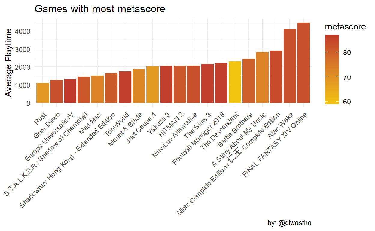
ggplot(data = video_game %>% group_by(max_owners) %>%
         arrange(desc(max_owners)) %>% head(10)) +
  geom_col(aes(x = reorder(game, max_owners), y = max_owners)) +
  labs(
    title = "Most Sold Video Games", y = "Number of copies sold", x = NULL,
    caption = "by: @diwastha"
  ) +
  theme_minimal() +
  theme(axis.text.x = element_text(angle = 45, hjust = 1))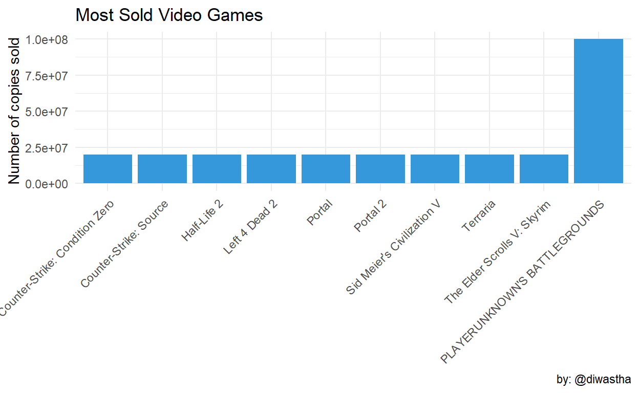
Dota2, Team Fortress 2 is free to play multiplayer games released on 2013 and 2007 respectively. The Player Unknown BattleGround(PUBG) is also a multiplayer battle royale shooter which is a huge hit. Counter-Strike is currently available free in steam which may have increased the owner count. All Top five games are multiplayer games with a strong player base and metascore.
ggplot(data = video_game %>% group_by(max_owners) %>%
         arrange(desc(max_owners)) %>% head(10)) +
  geom_col(aes(x = reorder(game, price), y = price, fill = price)) +
  labs(
    title = "Price of most sold games", y = "Price in $", x = NULL,
    caption = "by: @diwastha"
  ) +
  theme_minimal() +
  theme(axis.text.x = element_text(angle = 45, hjust = 1))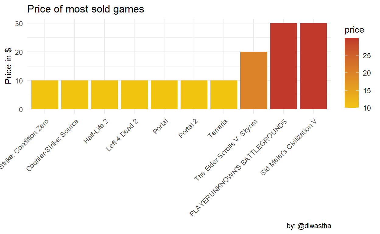
Pubg is currently one of the most popular games in the steam store and huge player base. Other games in this group have a very low price or currently free in the steam store.
ggthemr("flat")
ggplot(
  data = video_game %>% group_by(year) %>%
    summarise(avg_price = mean(price)),
  aes(x = year, y = avg_price)
) +
  geom_line() + geom_point(color = "red") +
  labs(
    title = "Average Price of the Game over the year",
    x = NULL, y = "price in $", caption = "by: @diwastha"
  ) +
  theme_minimal()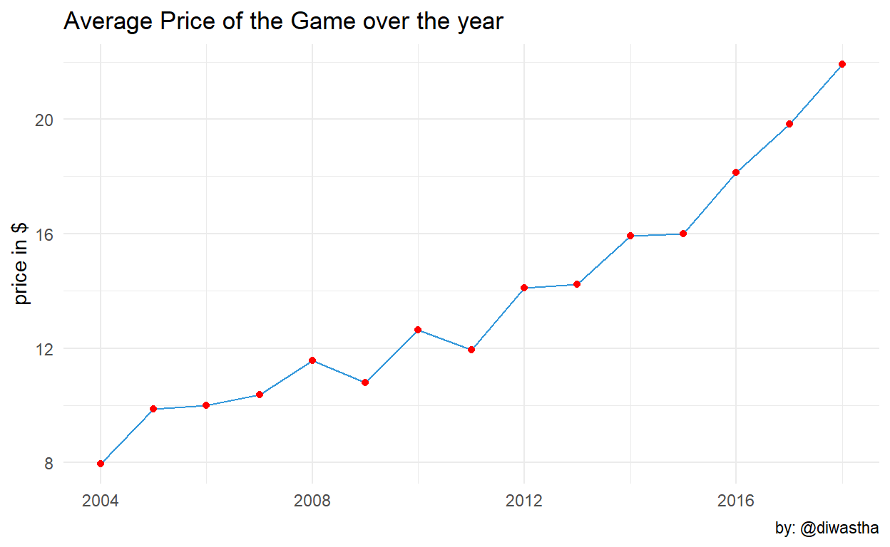
The average game price was rising up to the year 2013 then it started to decrease. It may be due to the increment in the release of the game with a very low price or freemium model.
ggplot(data = video_game) + geom_bar(aes(x = year)) +
  labs(
    title = "Number of active games since release year",
    y = "Number of Game", x = NULL, caption = "by: @diwastha"
  ) +
  theme_minimal()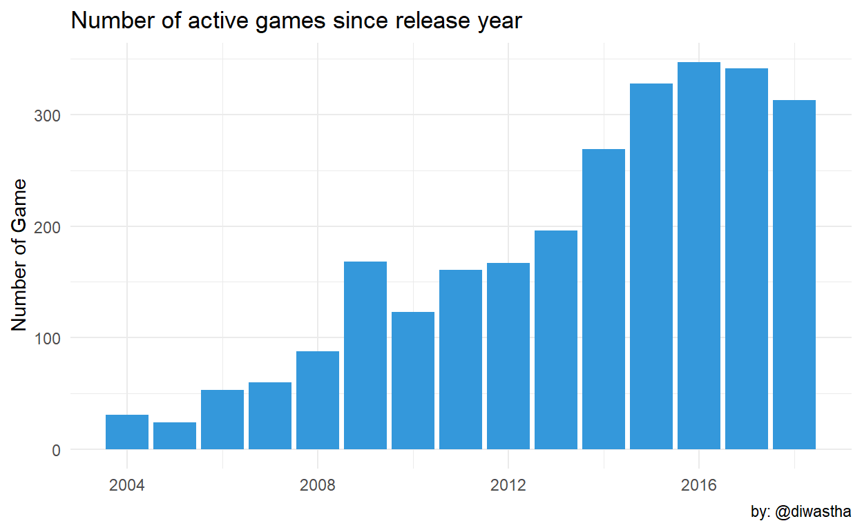
There is growth in the release of the games from the year 2015 onward.
ggplot(data = video_game) + geom_bar(aes(x = month)) +
  transition_time(year) +
  labs(
    title = "Games released in each month",
    subtitle = "Year: {frame_time}",
    y = "Number of Game", x = NULL, caption = "by: @diwastha"
  ) +
  theme_minimal()
The above animation shows the number of games released on each month of the year.
Wrapping up
Tidytuesday repo has a great dataset for analysis and visualization. You can also extract other data from the repo and work on it. I have taken some references from the work of other people while working on this data and they are: Anasthsia Kuprina CHRISTOPHER YEE